Experiencing Knowledge from Multiple Teachers

I am back with another tale of my colorful grad student days. This one happened sometime around end of 2017 when people were using Caffe (yes that Caffe) and Tensorflow was still being used for serious projects. PyTorch had just released their v.0.0.1 and it was ideal for beginners like me who ran off like scared puppies at the sight of Tensorflow or Caffe code…

At that time people were fascinated with deep networks. Everyone wanted to see how deep and wide we can make them. However, I had undertaken a research project which required me to port a deep CNN on an iPhone 6 (before they had “neural engine”). I saw that a simple CNN with a VGG-11 backbone could drain the battery of such a phone from $100%$ to $5%$ in a matter of minutes. Thus, I became interested in the question of compressing neural networks so that they can be reasonably run on edge devices.

In this blog post, I will introduce the field of model compression and touch on some related research that was done from the 90s to early 2016. Then, I’ll introduce an extension that I made to Hinton’s Knowledge Distillation framework and show that knowledge distillation worked really well when extended to the case of multiple teachers.

Model Compression

Let us imagine having some dataset $\mathcal{D_{train}} = \{\mathbf{x_i}, y_i\}_{i=1}^{n}$ on which we fit a model $f(\boldsymbol{\theta})$. We measure the performance of this network by computing some metric over unseen data $\mathcal{D}_{test}$ (typically it’s accuracy or F1-score).

The central question in model compression is this: Suppose I somehow come up with a model $f(\boldsymbol{\theta}’)$ such that $\boldsymbol{\theta}’ \subset \boldsymbol{\theta}$. How can I ensure that the model $f(\boldsymbol{\theta}’)$ has comparable performance to the original model?

At first glance, this question appears to be idiotic. If we replace the trained parameters $\boldsymbol{\theta}$ with a subset, we’re effectively performing a lobotomy on the network. Expecting very little performance drop is like expecting a lobotomized person to regain normal healthy function. However, we can do better than simply deleting some parameters and calling it model compression.

Saliency Based Methods

In the 90s, this question was taken up for shallow neural networks in two different works. Optimal Brain Damage (OBD)¹ considered the change in the objective function (called energy $E$) when the parameter $\boldsymbol{\theta}$(assumed to be already at a local minima) is perturbed by a small $\Delta$ i.e. $\theta_i’ = \theta_i + \delta_i$. The change is expressed as: $$ \delta E = \sum_i g_i \theta_i + \frac{1}{2}\sum_i h_{ii} \theta_i + \frac{1}{2}\sum_i \sum_j h_{ij} \theta_i \theta_j + O(||\delta \boldsymbol{\theta}||^3) $$

Here $\theta_i$ is the $i^{th}$ component of the parameter vector. $g_i$ is the element of the gradient $g_i = \frac{\partial E}{\partial \theta_i }$. The quantity $h_{ii}, h_{ij}$ are components of something called a Hessian. This is a matrix that captures the gradient of the gradient (e.g. if you have a function $f(x)=x^2$ then Hessian will be $f’(f’(x)) = 2)$. Now, since $\boldsymbol{\theta}$ is already at convergence, we can neglect the first term in RHS. Lecun et al make the assumption of a “diagonal” Hessian and thus ignore the third term in the above expansion. Thus, in their work $\delta E \approx \frac{1}{2}\sum_i h_{ii} \theta_i$. This means that the small change in $E$ can be computed readily during backpropagation. This $\delta E$ is called saliency of a parmeter towards $E$. Intuitively, it is a measure of how much contribution the parameter makes towards minimization of $E$. By computing the saliency for each parameter we can remove the least salient ones.

A derivative of the OBD algorithm was called Optimal Brain Surgeon (OBS)². It derived a different form of saliency $L = \frac{1}{2}\frac{\theta_q^2}{[\boldsymbol{H}^{-1}]_{qq}}$ where $q$ is the index of the parameter to be pruned. The algorithm requires computation of $\boldsymbol{H}^{-1}$ until convergence and the authors provide a recursive iterative algorithm for calculating this quantity. While it was more accurate then OBD in identifying redundant parameters, it was also slower. The full derivation and discussion is quite interesting in and of itself but is outside the scope of this blog post.

Compression Pipelines

Saliency based algorithms had the drawback of not being scalable when considering billions of parameters. An alternative approach was provided by the Deep Compression³ paper:

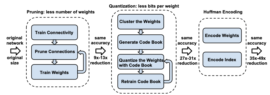
The deep compression pipeline has three stages: Pruning, Quantization and Huffman Encoding. In the pruning stage, the parameters below a threshold are. eliminated. The network is retrained to allow the remaining parameters to adapt to the original data. The quantization stage cleverly groups the weights of into buckets which are indexed by centroids. Weights within the same neighborhood of their centroid are assigned the same “bucket”. The gradients are also grouped in their respective buckets and the updates are applied to these quantized representations of weights. Huffman encoding is a greedy compression algorithm that is finally applied to the pruned and quantized networks to save space. The results reported by authors on fully connected and CNN architectures on MNIST and Imagenet are pretty impressive. For example, this result shows that their pipeline achieved 39-49x parameter reduction:

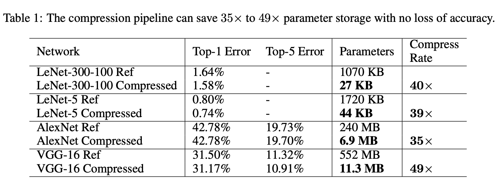
You can refer the paper for more in-depth discussion but the point is that even for deep neural networks there exist some really clever ways to prune network parameters.

Knowledge Distillation

There was a different line of work proposed by Hinton et al⁴. Unlike previous and related works that tried to compute weight saliency after the network had been trained, their method (dubbed Knowledge Distillation) proposed to transfer knowledge between two neural networks of different sizes.

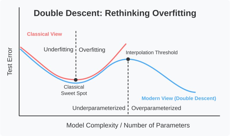
Before diving into the formulation, let’s take a step back and think as to why this method should work? As any practitioner of machine learning will tell you, there is an underfitting and overfitting regime in deep neural networks. However, beyond a certain threshold, the overfitting turns into interpolation. In simpler terms, a massively overparameterized model begins to draw connections between seemingly unconnected data points. This means that within the parameter space of a large model, there exists a compact but powerful representation of data that allows it to reason about unseen data. If we can somehow “teach” a smaller network to learn from this large network, then intuitively it’s performance should also increase.

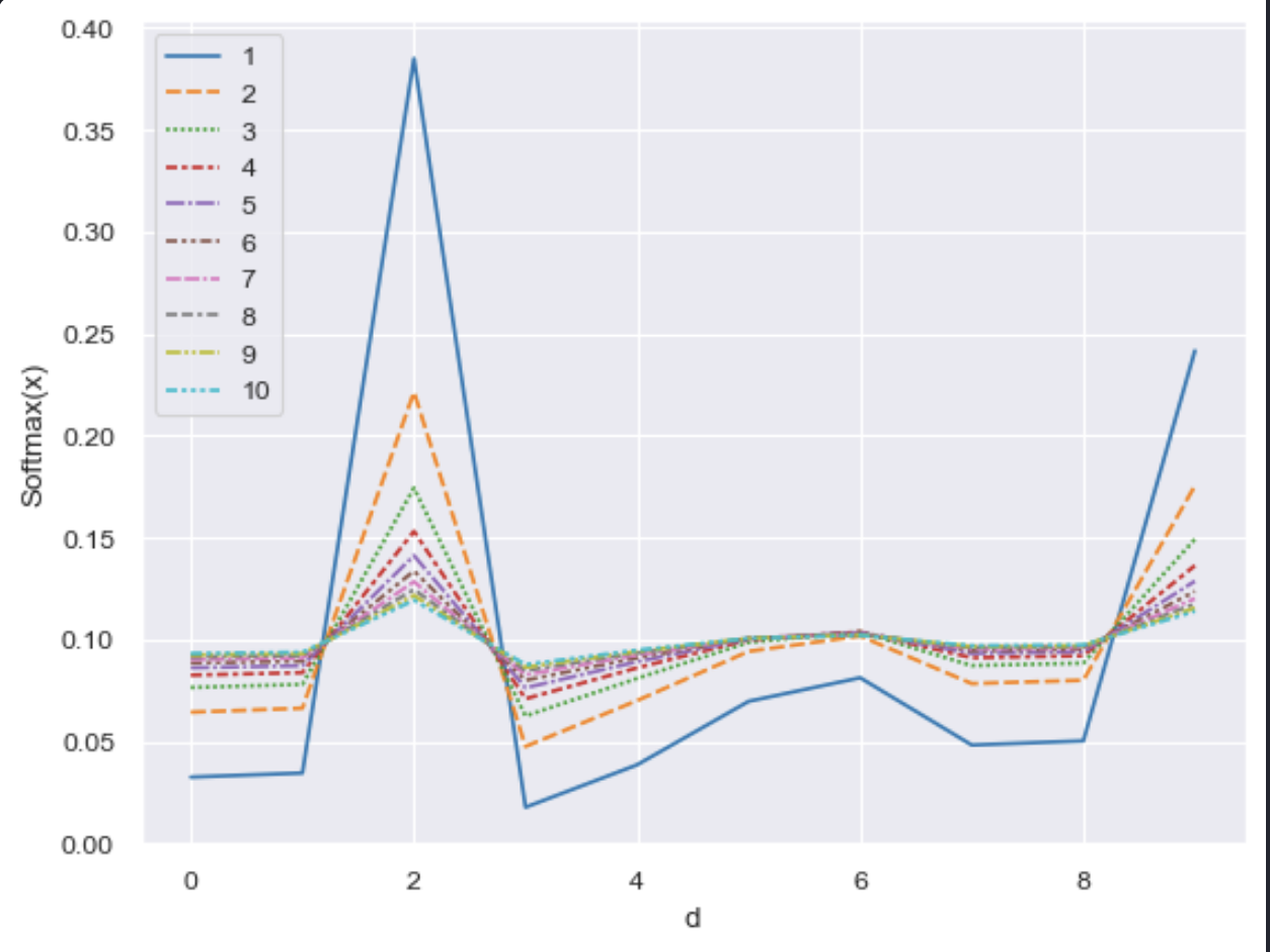
Typically in a neural network we apply a softmax to “squash” the output logits $\mathbf{z} \in \mathbb{R}^d$ into a probability i.e. $p_i = \text{Softmax}(z_i) = \frac{e^{z_i/T}}{\sum_{j=1}^d e^{z_j/T}}$. The $T$ term can be tripping for a lot of people. We call this a temperature parameter. It is usually set to $1$ for typical training.

Hinton et al hypothesized that setting $T > 1$ effectively “softens” the probability distribution produced by a neural network (in response to an input $\mathbf{x}_i$). The figure below shows the softening effect on a simulated logit (drawn from $\mathcal{N}(0, I) \in \mathbb{R}^{10}$) when $T$ is varied from $1 \mapsto 10$. You can see the weight of softmax gradually diminishing and “spreading out” over other possible values. Thus, instead of encoding the belief over the most likely output value, a teacher network with softened softmax produces a belief distribution over all likely output values.

Now let’s examine what happens when we try to train a network by taking these softened logits as targets for a smaller network. The loss function is Cross Entropy: $$ \mathcal{L} = -\sum_i p_i \log(q_i) $$

The gradient w.r.t to student logit $z_i$ is:

$$ \frac{\partial \mathcal{L}}{\partial z_i} = \frac{1}{T}(q_i - p_i) = \frac{1}{T}(\frac{e^{z_i/T}}{\sum_{j} e^{z_j/T}} - \frac{e^{v_i/T}}{\sum_j e^{v_j/T}}) $$

Here $v_i$ is the logit in the teacher model. If we assume,$|z_i| « T$ and the inputs to be zero meaned, then the gradient will simplify to:

$$ \frac{\partial \mathcal{L}}{\partial z_i} \approx \frac{1}{NT^2}(z_i - v_i) $$

The approximation tells us that the error backpropagated to the student model is the distance from the temperature softened logits of the teacher model. Hinton et al proposed a loss function that combined the cross entropy loss between the student model’s output and the ground truth labels (“hard targets”) and the cross entropy loss defined above. They found doing so allowed a student model to learn about representations even if there are some labels missing in the training data.

This approach to model compression is different from what we saw earlier. Instead of trying to operate on a previously trained model, this approach simply trains a smaller model that absorbs the knowledge from a larger model (and training data if avaialable).

Experience Loss

Hinton et al hypothesized that their framework could be extended to an ensemble of teacher models. At first glance, the extension seems trivial since we only need to add more terms to the “soft” CE loss. However, the question is more subtle than it appears. This is primarily due to two reasons:

1. Different teacher models have different “capacities”. Thus, they may produce logits that vary considerably in magnitude. The the difference in logits is consistently high, then we can call the teacher and student to be incompatible. Simply training a CE-like loss for multiple teachers can then even harm training.

2. The temperature regimes for different teachers will also vary. We need to ensure that the logit matching from one teacher does not always dominate the training.

Given these considerations, I proposed the Experience Loss formulation:

$$ \mathcal{L_{\text{EKD}}} = \mathbb{E}[\sum_{j=1}^{|E|}KL(\hat{q}_i, \hat{p}_j) - y_i \log(q_i)] $$

Here $E$ is the total number of teacher models in the ensemble. $\hat{q_i}$ is the probability produced by a student model. It is softened by $T_{student}$. $\hat{p_j}$ is the softmax produced by model $e_j \in E$ softened by it’s temperature $T_j$. The second term in the loss is the CE loss between the un-softened probability and the “hard target”.

If we consider the gradient of the first term in this loss function for a single teacher model $e_j$, we will obtain:

$$ \frac{\partial \mathcal{L_{\text{EKD}}}}{\partial z_i} \approx \frac{1}{NT_{student}}(\frac{z_i}{T_{student}} - \frac{v_j}{T_j}) $$

Here, the point about compatibility becomes more clear. If we fix $T_{student} = T_j$ then the only focus is on matching logits between two models. There’s little we can do besides empirically select the most compatible models in an ensemble through empirical studies. However, having access to varying temperatures, allows us to take any arbitrary teacher network and adjust it’s logits so that they don’t overwhelm the student logits. Moreover, we can also adjust student logit temperature to ensure compatibility.

Experiments with Experience Loss

To study how Experience Loss helps in knowledge transfer from multiple teachers I ended up developing two student architectures. I called them the WideShallow and WideDeep architectures. The basic building block of the WideShallow block is shown below:

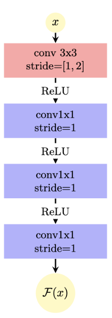
Notice how the block mostly has $1 \times 1$ convolutions? This is intentional since I want the parameters to be less. The initial block has a wider convolution window because we need to process the feature maps for greater context. The network had 5 layers and a total size of only $2\text{MB}$ (roughly $161K$ parameters). To study the effect on a more parameter heavy but still shallow network I introduced the WideDeep architecture that has two different blocks:

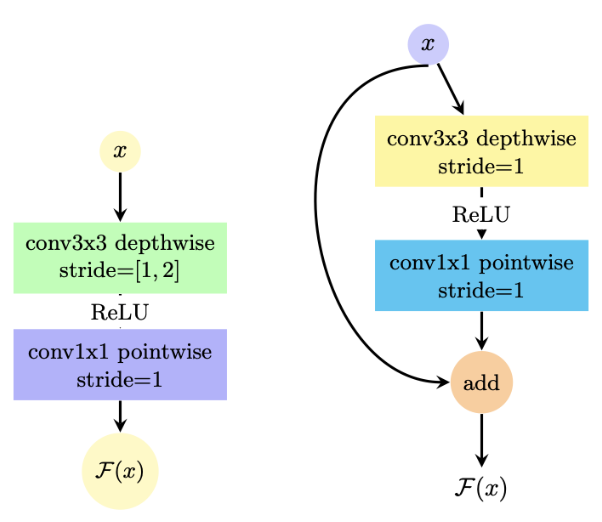
The left block is used in “entry” and “exit” (i.e. the layers closest to input and just before linear projection). The right block is used in the middle part of the network. It is inspired by the ideas of separable depthwise convolutions. This architecture (5 layers) has a size of $18\text{MB}$(roughly $4.53M$ parameters).

In distilliation loss there’s only one hyperparameter to tune. In my formulation however, there is a set of hyperparameter. More importantly, to ensure that knowledge transfer from a teacher to student can happen we need to set the student temperature $T_{student}$ appropriately. I proposed three strategies to do this automatically by three functions $F=[f_{mean}, f_{min}, f_{max}]$. Essentially:

$$ T_{student} = f_i(\mathbf{T}); \forall f_i \in F $$

I trained a WideshallowNet architecture on CIFAR-10 dataset with different teacher architecture and ensembles. The baseline student architecture was trained without any teacher influence. These were the results:

You can see setting $T_{student}$ to the minimum of all teacher temperatures worked extremely well. Also, I noticed that any temperature beyond $T>30$ was a decreasing RoI in thie technique.

To see the effect of experience loss on standard shallow CNNs, I trained a shallow CNN student model on Google’s SVHN dataset. The results are shown below:

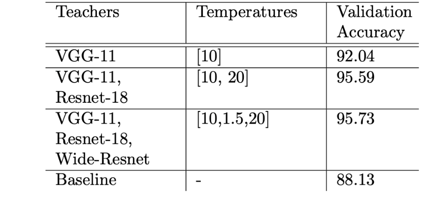
In the case of single teacher, I used the Distillation Loss as the training loss function. You can see that the accuracy is significantly boosted when using an ensemble of teachers. The bigger the ensemble the higher the accuracy. The temperature values were found by performing a grid search on values ranging from $T=1 \dots 30$.

Finally, we are interested in how much model compression can we achieve with this technique. In saliency based and pipeline based approaches, we can simply compute the ratio between input and output models. However, in distillation cases we are forced to come up with a different definition of compression ratio. I defined it as follows:

$$ \phi = \frac{\sum_{i=0}^N \Omega(m_i)}{\Omega(s)} $$

Here $\Omega(m)$ is the total memory consumption of a single network $m$. The sum in the numerator is reasonable since with experience loss we are using a single model in place of the entire ensemble on the same dataset. The compression results are shown below:

Extensions to Experience Loss

This formulation is from over 8 years ago. A lot of new techniques have emerged since then. However, this part is where I discuss what I think about extending this work.

One key thing that both distillation and experience losses ignore is the gradient information during training a student model. I think that temperature should somehow incorporate this information during student training to ensure that the knowledge transfer is effective throughout training and not just in the beginning. One can think of adding a momentum like term like in ADAM⁵ optimizer. Thus, for a single teacher/student case we can have:

$$ T_0 \gets T_{init} $$ and then $$ T_{t} \gets \gamma T_{t-1} + (1-\gamma)g_{t}^s $$

Where $g_t^{s}$ is the gradient of the student network’s parameters at time step $t$. The procedure can be easily extended to the case of multiple teachers.

Conclusion

The era of really large models is upon us. As they grow to handle greater context sizes and multimodal data there is always a fear that at some point they may hit the upper limit of energy and memory consumption. Already, the datacenters run by Amazon, Microsoft etc consume more energy than some rural areas of the US. Model compression has a rich history of techniques and the question it tries to solve was relevant in the 90s and is still relevant today. Perhaps, by introducing some novel ideas in this direction in the future, we may be able to reap the benefits of AI without worrying about the impending compute and memory wall.