Randomized Measurements and Shadows (a.k.a Part 2)

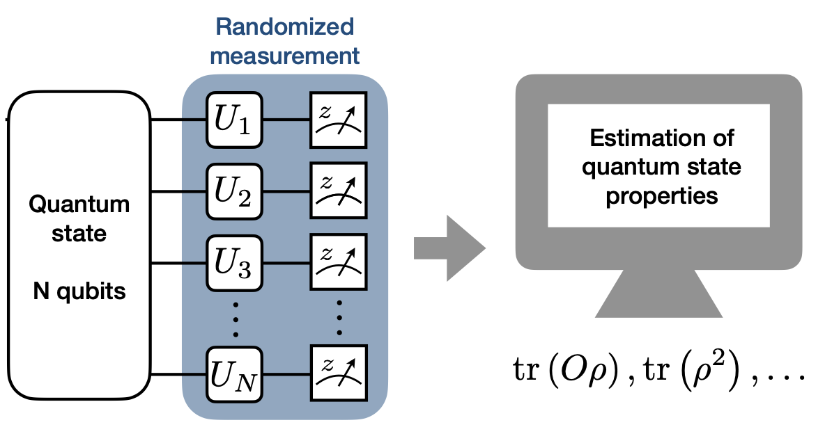
In the earlier blog post I had described the an interesting piece of quantum information science literature - classical shadows. The overreaching idea was to use random measurements to obtain some information about an unknown quantum state without requiring to store (or know) multiple copies of that state and re-construct it. Classical shadows have two advantages when it comes to today’s state of quantum computing. First, they are measurement efficient i.e. they allow us to reconstruct any quantum state and make predictions on those independent of the system size (i.e. the number of qubits in the state). Second, they provide us a way for mapping a quantum quantity (heh) to something that can be handled by existing computers (classical computers).

In this post, I am going to make the empirical protocol much more precise and discuss the applications that arise due to the second property of classical shadows. At the end of this post, I hope to convince you to pay a closer look at classical shadows and think of interesting ways you can incorporate quantum computers in your optimization tasks or vice versa.

Much of the material for this post is derived from a seminal paper by Elben et al. Many of the pictures in this blogpost are from that paper as well.

Randomized Measurements: Measurement Protocol

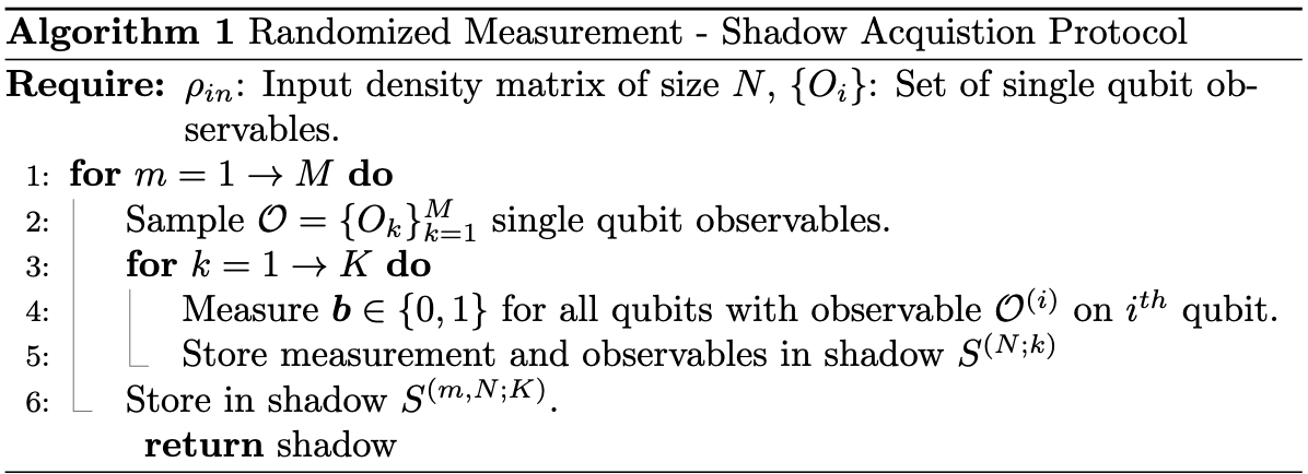
The first step in classical shadows is to acquire shadows from an unknown quantum state $|\psi\rangle \in C^{\otimes n}$. In order to do so with randomized measurements, we use the following algorithm:

Here, in the worst case we use $O(MKN)$ time and memory to acquire and use the shadows. This may seem a lot, but it is relatively cheaper than requiring to store $O(K. 2^{N} . 2^{N})$ copies for a full state tomorgraphy. However, these asymptotics are in the worst case. Many times we can get away with keeping $M, K$ to a reasonably large value and save on both time and memory. This is because our goal in classical shadows is not to perform a full shadow tomography(it is, but it’s not what makes them super useful) but to predict properties of many observables simultaneously.

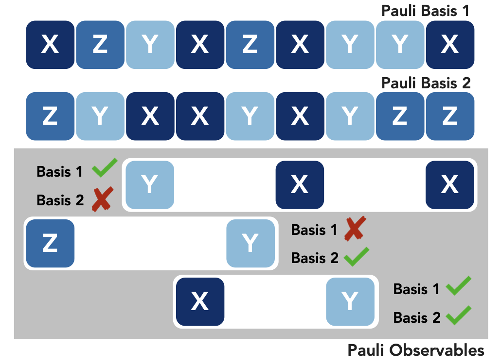
We can consider two extreme cases and see the usefulness of the protocol. First, when $M=1$, we sample an observable once during the entire acquisition process and repeat the measurement $K$ times. When a shadow is obtained in this manner, we can predict linear values like $Tr[O\rho]$ for different $O$ provided they are in the exact same basis as the sampled observable. For instance, let’s say for a 3-qubit system the sampled observable was $X \otimes Z \otimes Z$. Then, we can predict observables of the form $\alpha X \otimes \beta Z \otimes \gamma Z$ for different values of $\alpha, \beta, \gamma$.

The first case is fun, but limits us to a single observable that we sampled at random. When we do the opposite i.e. $K=1$ it means that we will sample $M$ different observables and the shadow will be a measurement in those $M$ different basis. Going back to our 3 qubit example, lets say we sampled $Z \otimes Z \otimes X$ , $X \otimes X$, $Y \otimes Z \otimes X$ and acquired the shadow. Then we can measure values for $Tr[O\rho]$ for any $O$ that has a matching basis on that qubit. In this case, we sacrifice the accuracy of obtaining a shadow for a basis to be able to combine expected values from an ensemble of diverse observables. A situation like this is shown in the picture:

Computing the values of $M$ observables and reconstruction of the shadow $\hat{\rho}$ is same as described in the previous blog post. I’ll restate these succintly in equation form here:

$$ \hat{o} = \frac{1}{M}\sum_{m=1}^{M} tr(O\hat{\rho}^{(m)}) $$

$$ \hat{\rho}^{(m)} = \frac{1}{K}\sum_{i=1}^{K} \bigotimes_{n=1}^{N} (3(U_n^{(m)})^{\dagger}|s^{m,k}_n\rangle \langle s_n^{(m, k)}| U^{(m)}_n - \mathbb{I}) $$

Applications of Classical Shadows

Once we’ve construted our fighter plane, let’s see what it can do.

Classical Shadows as Data Format

Since classical shadows act as a way to map quantum to classsical information, we can use them as a data format for many downstream applications. In the RMT paper, the authors propose to use the information provided by a classical shadow $S^{(M, K,N)}$ as data to train a machine learning model for detecting topological entanglement entropy for different kinds of quantum models.

In the paper, the authors consider detecting this non-linear entropy for an XXZ model and toric code topological phase. The exact description of these systems is beyond the current scope of this post, and I’ll stick to the results:

These results show very interesting things. First, in the left plot we can clearly see that the shadow obtained from a quantum system has a natural clustering in classical space even when the number of measurements are finite. Second, in the right plot we can see that a shadow provides important a-priori information to a classical machine learning algorithm and enables it to perform a discriminative classification much more effectively as compared with just training on a raw quantum data.

Quantum Fidelity Estimation

One of the most important quantities in quantum information science is fidelity. In simple terms, it estimates the degree of closeness for any two quantum states. The classical analog of fidelity is the cosine distance in Euclidean space. In classical ML tasks, we typically can access two vectors $\textbf{x}, \textbf{y}$ in polynomial time and thus compute the cosine distance efficiently.

The same is not true for quantum states since the only way to access an unknown quantum state is to reconstruct that state and then estimate the fidelity. Needless to say, this procedure does not scale for large system sizes. Moreover, there are two kinds of fidelity estimation we are interested in performing:

1. Maximum Fidelity Estimation: Estimate correlation between two arbitrary states $\rho_1, \rho_2$

2. Direct Fidelity Estimation: Estimate the overlap between a pure quantum state $|\psi\rangle$ and a unknown given state $\rho$ (most likely prepared with imperfect instruments).

Classical shadows to the rescue! Let’s first consider the case of maximum fidelity estimation. We’re interested in the quantity:

$$ \mathcal{F}_{max} = \frac{Tr[\rho_1\rho_2]}{max[Tr[\rho^2_1], Tr[\rho^2_2]]} $$

The bottleneck is the reconstruction of $\rho_1, \rho_2$ directly. We use the randomized measurement protocol to estimate $S_1(M, K, N)$ and $S_2(M, K, N)$. Since we know that this shadow reconstructs the input state in expectation, we can compute a statistical correlation (e.g. Pearson correlation, Spearman correlation) that will give us $Tr[\rho_1, \rho_2]$ by proxy. A large value of correlation coefficient will indicate a large overlap while a value of 0 will indicate two completely different systems.

The case of direct fidelity estimation is a bit more challenging since we have a known pure state $|\psi\rangle$ and an unknown quantum state $\rho$. The fidelity given as $Tr[\rho\psi]$ cannot be approximated by proxy like a statistical correlation since one system is known. Instead, the authors in the paper propose to proceed as follows:

Write $\rho = \sum_j a_j Q_j$ where $Q_j \in {I, X, Y, Z}$ and $|\psi\rangle = \sum_j b_j Q_j$. Then

$$ \mathcal{F}(\rho, \psi) = \sum_j a_j b_j = \sum_j (\frac{a_j}{b_j}) b^2_j $$

The expansion of states can be understood as writing them in terms of weighted Pauli coefficients. The equality then arises since $Q^2_j = 1$. The last expression can be interpreted as an expectation over a known distribution $b_j$ with a random variable being the ratio of coefficients between known quantum states and unknown state. With classical shadows we can estimate $\mathcal{F}$ upto an accuracy of $\varepsilon$ by sampling $O(\frac{1}{\varepsilon^2})$ observables from the distribution of $b^2_j$ and estimating $Tr[O\rho]$. We know classical shadows allow us to do this independent of system size and in logarithmic time :)

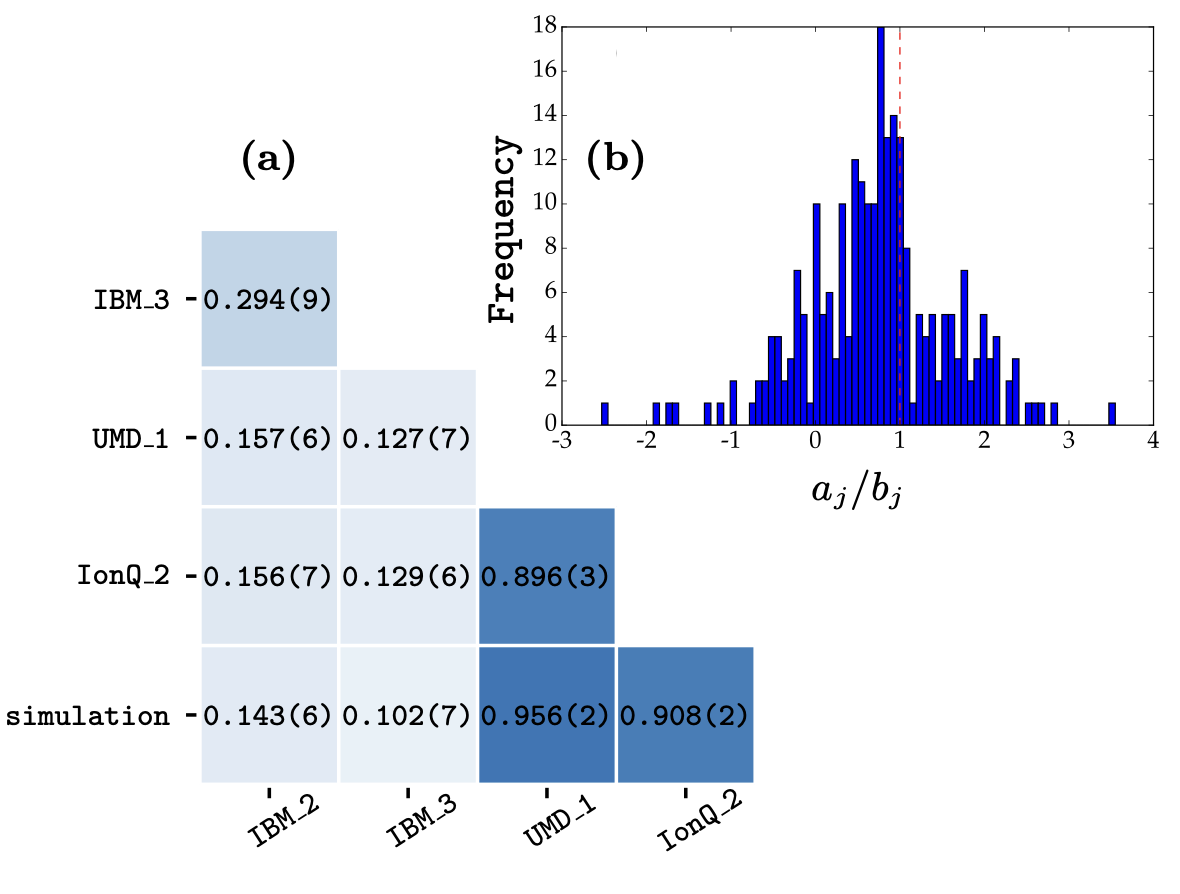
A result for estimating fidelity with a 7 qubit GHZ state on various IBM devices and Ion-trap devices shows that we can indeed estimate the fidelity values efficiently. Part (a) shows the cross device fidelity on various devices and (b) shows the distribution of the random variable $(\frac{a_j}{b_j})$ for a 14-qubit quantum state.

Variational Quantum Algorithms (VQAs)

VQAs are currently heavily researched in quantum computing since they promise to help us leverage a (hypothetical) quantum computer in the near future. The typical way of training a VQA is to instantitate parameters on a classical computer and use them to estimate measurement for some observable on a quantum computers. The paramters are updated using gradient descent like procedure.

Quantum circuits are composed of unitary matrices that are applied to some input quantum state $|0\rangle$ to produce some mixed output state $\rho_{out}$. Typically, these unitary matrices are represented as gates in a circuit (much in the same way we’re used to seeing digital gates like AND, OR, NOT except these are analog gates). Variational quantum circuits add a real valued parameter $\theta$ to each gate. We can think these circuits in terms of layers where unitarites are applied one after the other:

$$ U(\vec{\theta}) = \prod_{l=1}^L U(\theta_l) $$

In a very crude way, these quantum circuits can be interpreted as linear networks whose real valued weights are optimized for a given cost function $C(\theta)$ on a classical computer. In simpler terms, we can think of these circuits running some analog quantum computation with given parameters on a quantum computer that’s attached as a co-processor and the parameters themselves are being adjusted on the main CPU.

Now that we’ve successfully distilled the power of known universe to our desktop computation, it’s time to look at what cost function we’re optimizing. Typically, the cost function we’re interested in is of the form:

$$ C(\vec{\theta}) = Tr[U(\vec{\theta})O\rho_{in}U^{\dagger}(\vec{\theta})] $$

Here $O$ is the observable we’re interested in predicting. $U(\vec{\theta})\rho_{in}U^{\dagger}(\vec{\theta})$ is the output quantum state produced by the action of the quantum circuit. If you’ve followed along thus far, there should be a gleam in your eyes and a smirk on your face since this cost function is very similar to the form $Tr[O\rho]$ which we know we can estimate efficiently using classical shadows. In fact, classical shadows enable us to do something better - We can estimate $C_{1}(\vec{\theta}), C_{2}(\vec{\theta}) \dots C_{M}(\vec{\theta})$ in parallel for $M$ observables in $\sim O(log M)$ time!

Given the utility of classical shadows in this scenario, there are lots of ways they have been explored in recent literature. I’m going to look at some interesting examples that represent the possibilites in the NISQ era:

1. Alternating Layered Variational Quantum Circuits Can Be Classically Optimized Efficiently Using Classical Shadows Basheer et al: Leverage classical shadows to reduce the number of function evaluations in an alternating layer ansatz and single qubit observables. Their proposed approach reduces the number of function evaluations for $L$ steps to $~\sim O(log L)$ from $O(L)$.

2. Avoiding Barren Plateaus using Classical Shadows Stefan Sack et al: VQAs suffer from a pain in the ass called barren plateaus. They are regions on optimization surface where the mean of gradients converges to zero and variance decays exponentially with increasing system size. In this paper, the authors characterize weak barren plateaus as a point where the Renýi entroy $S_2 = -ln\ tr[\rho^2_A] \geq \alpha S^{page}$. Where, $S^{page}$ is the entropy of the maximally scrambled state and is approximated as $S^{page} = K ln 2 - \frac{1}{2^{N-2K+1}}$ where $K « N$ and $A$ is the subsystem we’re interested in. Their proposal is to estimate $S_2$ using shadows during optimization for some value of $\alpha \in [0, 1)$ and adjust the learning rate accordingly.

3. Training variational quantum circuits with CoVaR: covariance root finding with classical shadows: Traditional VQE algorithms seek to find the ground state associated with a Hamiltonian of a molecule. This ground state typically is some eigenstate of the Hamiltonian, estimated via parameter optimization. In this paper, the authors propose to find this eigenstate by estimating covariance between the problem Hamiltonian and their chosen set of observables. In order to do so at scale, they propose to use shadows to minimize calls to a quantum circuit and evaluate the necessary equations on the classical computer.

Conclusions

In these two blog posts, I’ve tried to present a picture on the usefulness of classical shadows in quantum information science. I’ve shown them to be useful in situations where quantum computation is cumbersome and one needs a way to process information using classical computers efficiently. I’ve given some examples of creative uses of shadows in near term quantum computers. Hopefully, if you’ve stuck with me so far you will be inspired to give a closer look to shadows and think of using them in any of your own projects.

Till next time!